Introduction
For this project, I’m going to run through an example of fitting a multiple linear regression model in R. We’re going to see if we can use this to accurately predict the price of Vintage Bordeaux wine each year based on a few measured variables for each vintage. To do this, we’ll use variety of statistical and visual methods to evaluate the model, as well as perform a transformation to see if that improves the fit. If you’re unfamiliar with any of the tests or methods I use, a quick Google search will yield numerous great resources for each concept.
First, let’s take care of some housekeeping by setting the working directory and importing the csv file:
## Set Working Directory
  setwd("/Users/Chris/Documents/R/Linear Model Evaluation and Transformation in R")
    getwd()
## [1] "C:/Users/Chris/Documents/R/Linear Model Evaluation and Transformation in R"
## Import Data
    data <- read.csv(file.path("Bordeaux.csv"), header = TRUE,sep=",")
    data
##    Year  Temp Rain PrevRain Age Price
## 1  1952 17.12  160      600  31 0.368
## 2  1953 16.73   80      690  30 0.635
## 3  1955 17.15  130      502  28 0.446
## 4  1957 16.13  110      420  26 0.221
## 5  1958 16.42  187      582  25 0.180
## 6  1959 17.48  187      485  24 0.658
## 7  1960 16.42  290      763  23 0.139
## 8  1961 17.33   38      830  22 1.000
## 9  1962 16.30   52      697  21 0.331
## 10 1963 15.72  155      608  20 0.168
## 11 1964 17.27   96      402  19 0.306
## 12 1965 15.37  267      602  18 0.106
## 13 1966 16.53   86      819  17 0.473
## 14 1967 16.23  118      714  16 0.191
## 15 1968 16.20  292      610  15 0.105
## 16 1969 16.55  244      575  14 0.117
## 17 1970 16.67   89      622  13 0.404
## 18 1971 16.77  112      551  12 0.272
## 19 1972 14.98  158      536  11 0.101
## 20 1973 17.07  123      376  10 0.156
## 21 1974 16.30  184      574   9 0.111
## 22 1975 16.95  171      572   8 0.301
## 23 1976 17.65  247      418   7 0.253
## 24 1977 15.58   87      821   6 0.107
## 25 1978 15.82   51      763   5 0.270
## 26 1979 16.17  122      717   4 0.214
## 27 1980 16.00   74      578   3 0.136
Part 1: Construct a Regression Model that Describes the Price of the Vintage
Let’s create a multiple linear model of the price of Vintage Bordeaux as a function of its Age (in years where 1983=0), Rainfall (mm during the harvest season), Previous Rainfall (mm in the six months before the harvest season), and Temperature (degrees Celius during the growing season).
y <- data$Price
x1 <- data$Age
x2 <- data$Rain
x3 <- data$PrevRain
x4 <- data$Temp

# multiple linear regression
fit <- lm(Price ~ Age + Rain + PrevRain + Temp, data = data)
Part 2: Run a Regression Analysis on the Data
Now we need to run a summary of the multiple linear regression to find the quantiles, coefficients, R-squared value, adjusted R-sqared value, F-Statistic, and the p-values. We’ll then run an ANOVA table to get the variance data.
summary(fit)
##
## Call:
## lm(formula = Price ~ Age + Rain + PrevRain + Temp, data = data)
##
## Residuals:
##      Min       1Q   Median       3Q      Max
## -0.14072 -0.08770 -0.01074  0.03410  0.26783
##
## Coefficients:
##               Estimate Std. Error t value Pr(>|t|)
## (Intercept) -3.1716289  0.6928899  -4.577 0.000147 ***
## Age          0.0080519  0.0029410   2.738 0.012013 *
## Rain        -0.0010351  0.0003314  -3.123 0.004947 **
## PrevRain     0.0005638  0.0001979   2.849 0.009338 **
## Temp         0.1903096  0.0390606   4.872 7.18e-05 ***
## ---
## Signif. codes:  0 '***' 0.001 '**' 0.01 '*' 0.05 '.' 0.1 ' ' 1
##
## Residual standard error: 0.1176 on 22 degrees of freedom
## Multiple R-squared:  0.7356, Adjusted R-squared:  0.6875
## F-statistic:  15.3 on 4 and 22 DF,  p-value: 4.017e-06
summary(aov(fit))
##             Df Sum Sq Mean Sq F value   Pr(>F)
## Age          1 0.2354  0.2354  17.025 0.000443 ***
## Rain         1 0.2614  0.2614  18.905 0.000258 ***
## PrevRain     1 0.0212  0.0212   1.532 0.228900
## Temp         1 0.3283  0.3283  23.738 7.18e-05 ***
## Residuals   22 0.3042  0.0138
## ---
## Signif. codes:  0 '***' 0.001 '**' 0.01 '*' 0.05 '.' 0.1 ' ' 1
Note the R-Squared value is only 0.7356, which means only 73.56% of the variance in price is predicted from the current model. This is not particularly high, and should make us question the efficacy of the current linear model.
Let’s also check the four model assumptions to see if the model is appropriate. These four assumptions are linearity, independence, normality of residuals, and equal variance of residuals.
Part 3: Check the Model Assumptions
## 1. check for linearity
layout(matrix(c(1,2,3,4),2,2))

## run simple plots with each variable to check for linearity
plot(y ~ x1, main = "Price vs Age", xlab = "Age (years)", ylab = "Price")
plot(y ~ x2, main = "Price vs Rainfall", xlab = "Rainfall (mm)", ylab = "Price")
plot(y ~ x3, main = "Price vs Previous Rain", xlab = "Previous Rainfall (mm)", ylab = "Price")
plot(y ~ x4, main = "Price vs Temperature", xlab = "Temperature (degrees C)", ylab = "Price")
## Residual Plots e_i vs x_i
par(mfrow = c(2,2))
plot(resid(fit)~x1, main = "Residuals vs Age",
     xlab = "Age (years)", ylab = "Residuals")
  abline(h = 0)
plot(resid(fit)~x2, main = "Residuals vs Rainfall",
     xlab = "Rainfall (mm)", ylab = "Residuals")
    abline(h = 0)
plot(resid(fit)~x3, main = "Residuals vs Previous Rain",
     xlab = "Previous Rainfall (mm)", ylab = "Residuals")
    abline(h = 0)
plot(resid(fit)~x4, main = "Residuals vs Temperature",
     xlab = "Temperature (degrees C)", ylab = "Residuals")
    abline(h = 0)
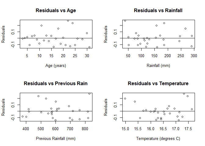
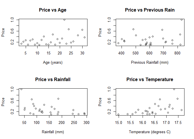
We see no evidence of linearity. There is not obvious relationship between any of the possible explanatory variables and the response variable (price) in any of the scatterplots. Furthermore, the patterns in the residual plots indicate that a linear relationship is not likely. We want to see a random distribution in the residual plots, which none of them have (the closest is price vs age, but it’s still clearly not random).
Next, we can run a Lag 1 Autocorrelation to see if the independence of errors is reasonable:
## 2. Check for Independence

##Lag 1 Autocorrelation
n = length(y)
acf(resid(fit), lag.max = 1, plot = FALSE)
##
## Autocorrelations of series 'resid(fit)', by lag
##
##      0      1
##  1.000 -0.588
2 / sqrt(n)
## [1] 0.3849002
Since 0.588 > 0.3849 independence of variables is not necessarily reasonable. This violates the second condition for linearity.
Next, we’ll checked for the normality of residuals with a q-q plot:
## 3. Check for normality of Residuals

# q-q plot
z <- ( fit$residuals - mean(fit$residuals) ) / sd(fit$residuals)
qqnorm(z, sub = "Residuals")
abline(a = 0, b = 1)
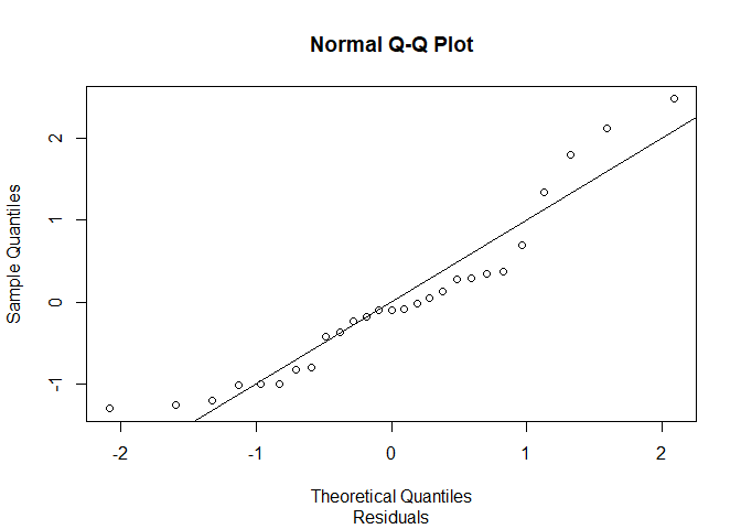
The q-q plot does not appear to be linear. We can say that errors are not necessarily normally distributed (it’s very likely that they aren’t).
Finally, we’ll check the equal variance of residuals with a plot of the residuals against fitted values:
# residual plots
layout(matrix(c(1,2,3,4),2,2))
plot(fit)
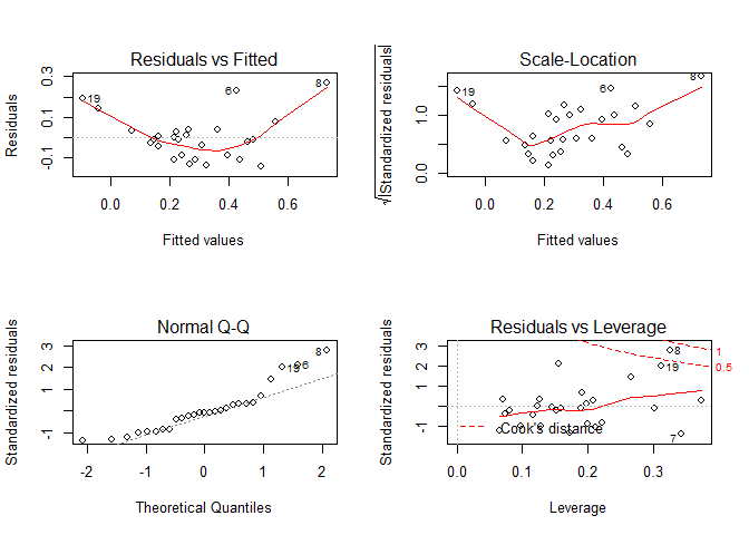
We see a pattern in the plot for the residuals vs fitted value, so it’s not likely that the errors have equal variances.
So, we have no evidence that our current model adheres to any of the four basic model assumptions. It appears the current model is not adequate.
Part 4: Transformation
To try and resolve this failure, we’ll apply a transformation to y. To perform the transformation, we can first run a box-cox power transformation to find the most appropriate transformation for y.
## Load additional library
    library(MASS)

# Plot of Log-likelihood function vs lambda
    boxcox(y ~ x1 + x2 +x3 + x4,
            plotit=T, lambda = seq(-2, 2, length = 10))
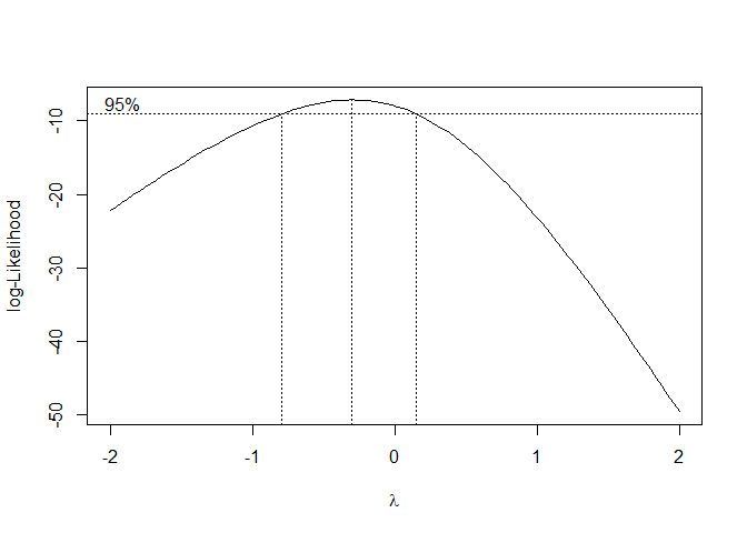
    ## Looking for lambda values 95% and above
    ## The "best" estimate for lambda is where the curve
    ## is at maximum (lambda approximately 0)
    ## A 95% confidence interval for lambda is
    ## approximately -1.3 to 1.3


## List of values of lambda and corresponding Log-likelihood function
    boxcox(y ~ x1 + x2 +x3 + x4,
            plotit=F, lambda = seq(0, 0.5, length = 10))
## $x
##  [1] 0.00000000 0.05555556 0.11111111 0.16666667 0.22222222 0.27777778
##  [7] 0.33333333 0.38888889 0.44444444 0.50000000
##
## $y
##  [1]  -7.938316  -8.287859  -8.701824  -9.180354  -9.723166 -10.329557
##  [7] -10.998429 -11.728321 -12.517450 -13.363766
    lambda <- 0


## Box-Cox power transformation
    trans.y <- log(y)
    trans.y ## transformed y values
##  [1] -0.9996723 -0.4541303 -0.8074363 -1.5095926 -1.7147984 -0.4185503
##  [7] -1.9732813  0.0000000 -1.1056369 -1.7837913 -1.1841702 -2.2443162
## [13] -0.7486599 -1.6554819 -2.2537949 -2.1455813 -0.9063404 -1.3019532
## [19] -2.2926348 -1.8578993 -2.1982251 -1.2006450 -1.3743658 -2.2349264
## [25] -1.3093333 -1.5417793 -1.9951004
y ## original dataset y values
##  [1] 0.368 0.635 0.446 0.221 0.180 0.658 0.139 1.000 0.331 0.168 0.306
## [12] 0.106 0.473 0.191 0.105 0.117 0.404 0.272 0.101 0.156 0.111 0.301
## [23] 0.253 0.107 0.270 0.214 0.136
## Linear regression of the transformated data
    trans.fit <- lm(trans.y ~ Age + Rain + PrevRain + Temp, data = data)
We pick the value of lamda with the largest log-likelihood (y-value). -7.938316 is largest and corresponds with approximately x = 0. So lamda = 0. This implies the best transformation for y is log(y).
Now we have an updated model. We’ll then apply the previous tests again to see if the results were better.
Part 5: Re-run Regression Analysis
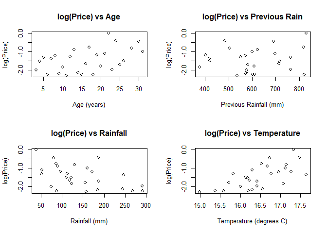
First, let’s look again at the simple plots for the new model to compare:
## 1. check for linearity
layout(matrix(c(1,2,3,4),2,2))

## run simple plots with each variable to check for linearity
plot(trans.y ~ x1, main = "log(Price) vs Age", xlab = "Age (years)", ylab = "log(Price)")
plot(trans.y ~ x2, main = "log(Price) vs Rainfall", xlab = "Rainfall (mm)", ylab = "log(Price)")
plot(trans.y ~ x3, main = "log(Price) vs Previous Rain",
     xlab = "Previous Rainfall (mm)", ylab = "log(Price)")
plot(trans.y ~ x4, main = "log(Price) vs Temperature",
     xlab = "Temperature (degrees C)", ylab = "log(Price)")
## Residual Plots e_i vs x_i
par(mfrow = c(2,2))
plot(resid(trans.fit)~x1, main = "Transformed Model Residuals vs Age",
     xlab = "Age (years)", ylab = "Residuals")
  abline(h = 0)
plot(resid(trans.fit)~x2, main = "Transformed Model Residuals vs Rainfall",
     xlab = "Rainfall (mm)", ylab = "Residuals")
    abline(h = 0)
plot(resid(trans.fit)~x3, main = "Transformed Model Residuals vs Previous Rain",
     xlab = "Previous Rainfall (mm)", ylab = "Residuals")
    abline(h = 0)
plot(resid(trans.fit)~x4, main = "Transformed Model vs Temperature",
     xlab = "Temperature (degrees C)", ylab = "Residuals")
    abline(h = 0)
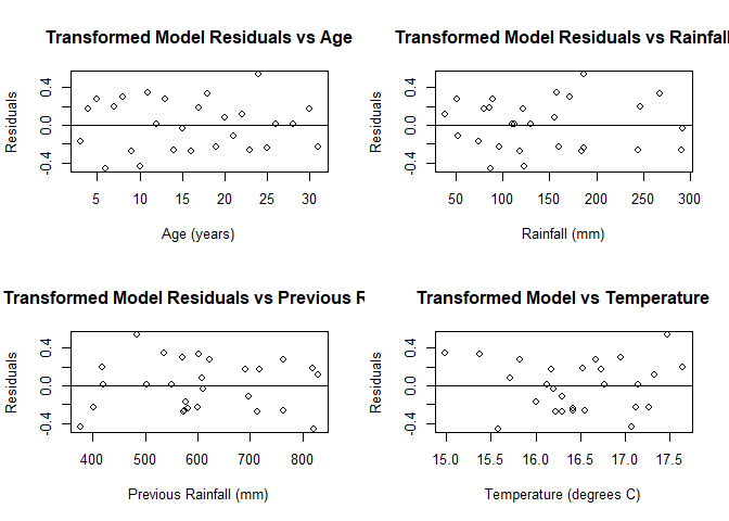
We see that the residual plots for age and rainfall appear to be without a pattern. Previous rainfall and temperature (especially temperature) may not be linear.
We’ll also take another look at the summary and ANOVA tables to get some quantitative information:
summary(trans.fit)
##
## Call:
## lm(formula = trans.y ~ Age + Rain + PrevRain + Temp, data = data)
##
## Residuals:
##      Min       1Q   Median       3Q      Max
## -0.45748 -0.23902  0.01067  0.18533  0.53642
##
## Coefficients:
##               Estimate Std. Error t value Pr(>|t|)
## (Intercept) -1.216e+01  1.686e+00  -7.213 3.15e-07 ***
## Age          2.390e-02  7.155e-03   3.341  0.00296 **
## Rain        -3.866e-03  8.062e-04  -4.795 8.66e-05 ***
## PrevRain     1.171e-03  4.814e-04   2.432  0.02359 *
## Temp         6.170e-01  9.502e-02   6.493 1.57e-06 ***
## ---
## Signif. codes:  0 '***' 0.001 '**' 0.01 '*' 0.05 '.' 0.1 ' ' 1
##
## Residual standard error: 0.2861 on 22 degrees of freedom
## Multiple R-squared:  0.8282, Adjusted R-squared:  0.797
## F-statistic: 26.51 on 4 and 22 DF,  p-value: 3.89e-08
summary(aov(trans.fit))
##             Df Sum Sq Mean Sq F value   Pr(>F)
## Age          1  2.224   2.224  27.178 3.15e-05 ***
## Rain         1  3.002   3.002  36.682 4.27e-06 ***
## PrevRain     1  0.003   0.003   0.038    0.847
## Temp         1  3.450   3.450  42.160 1.57e-06 ***
## Residuals   22  1.800   0.082
## ---
## Signif. codes:  0 '***' 0.001 '**' 0.01 '*' 0.05 '.' 0.1 ' ' 1
Note the increase of the R-Squared value to 0.8282 from 0.7356, which is a significant improvement. It’s worth noting that based on the p-values in the coefficients table, we can see that all four explanatory variables are significant.
We’ll run the Lag 1 Autocorrelation again to see if the independence of errors is reasonable for the new model:
## 2. Check for Independence

##Lag 1 Autocorrelation
n = length(trans.y)
acf(resid(trans.fit), lag.max = 1, plot = FALSE)
##
## Autocorrelations of series 'resid(trans.fit)', by lag
##
##      0      1
##  1.000 -0.417
2 / sqrt(n)
## [1] 0.3849002
Since 0.417 > 0.384, independence of variables is still not necessarily reasonable.
It’s time to check the normality of residuals assumption for the new model with a q-q plot:
## 3. Check for normality of Residuals

# q-q plot
z <- (trans.fit$residuals - mean(trans.fit$residuals) ) / sd(trans.fit$residuals)
qqnorm(z, sub = "Residuals (transformed)")
abline(a = 0, b = 1)
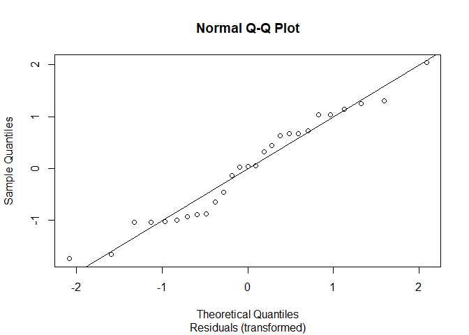
The q-q plot isn’t quite linear, so the results aren’t definitive. We can run a Shapiro-Wilk test for a more formal test to confirm:
    ## Shapiro-Wilk
  shapiro.test(trans.fit$residuals)
##
##  Shapiro-Wilk normality test
##
## data:  trans.fit$residuals
## W = 0.95865, p-value = 0.3441
With a p-value of 0.3441, we cannot reject the null hypothesis that the residuals are linear. Still, we’d be wise to doubt this is an optimal model as the we see a clear pattern to the q-q plot points.
Finally, let’s check for the equal variance of residuals with a plots of the residuals against fitted values:
# residual plots
layout(matrix(c(1,2,3,4),2,2))
plot(trans.fit)
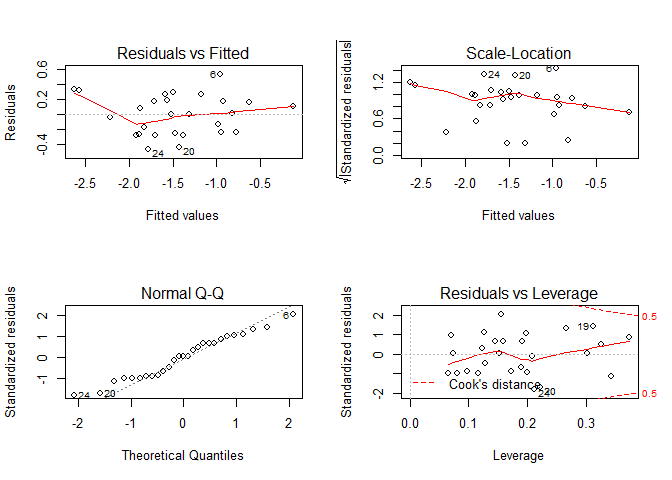
The residual plot appears to have no real pattern. It’s likely that the errors of this model have equal variances.
Overall, we see the new model is not perfect. However, it’s definitely an improvement.
Part 6: Analysis
As previously mentioned, the summary table for the log(y) transformed model showed that all four variables are significant, with the highest p-value being .024:
summary(trans.fit)
##
## Call:
## lm(formula = trans.y ~ Age + Rain + PrevRain + Temp, data = data)
##
## Residuals:
##      Min       1Q   Median       3Q      Max
## -0.45748 -0.23902  0.01067  0.18533  0.53642
##
## Coefficients:
##               Estimate Std. Error t value Pr(>|t|)
## (Intercept) -1.216e+01  1.686e+00  -7.213 3.15e-07 ***
## Age          2.390e-02  7.155e-03   3.341  0.00296 **
## Rain        -3.866e-03  8.062e-04  -4.795 8.66e-05 ***
## PrevRain     1.171e-03  4.814e-04   2.432  0.02359 *
## Temp         6.170e-01  9.502e-02   6.493 1.57e-06 ***
## ---
## Signif. codes:  0 '***' 0.001 '**' 0.01 '*' 0.05 '.' 0.1 ' ' 1
##
## Residual standard error: 0.2861 on 22 degrees of freedom
## Multiple R-squared:  0.8282, Adjusted R-squared:  0.797
## F-statistic: 26.51 on 4 and 22 DF,  p-value: 3.89e-08
The estimates column of the summary shows that Age, Previous Rain, and Temperature are positively correlated with price, and rain is negatively correlated with price. However, these values are extremely small (each change in one unit of the variable has a minimal effect on the log(price) when all variables are taken into condsideration).
All four of the basic model conditions are left with somewhat ambiguous results. This, combined with the R-squared value of 0.8282, which still leaves over 17% of the variance in price unexplained by the model, ought to make us question the adequacy of a linear model in the first place. It’s likely that some other model will more effectively model the effects of these variables on the price of Bordeax Vintage. However, if a linear model is required, the log(Price) transformed model is almost certainly the best.


